Alife/Statistical Extraction of Data from Visual Input

Input to Data Extraction Routine is multiple grayscale bitmaps, at least 1bit, 4bit, and 8bit maps; all represent same scene at same time. The first level of analysis uses the 1bit grayscale. The first “1” detected in a line by line check of said bitmap triggers the object recognition algorithm, as illustrated below.

The object recognition algorithm is as follows:

1) The Algorithm begins by evaluating the trigger pixel in relation to said pixel’s 8 adjacent pixels. If all 8 adj. Pixels are empty, Algorithm terminates and control is returned to Primary DER. DER proceeds to next “on” bit in pixel map.

2) The algorithm has three subtypes; high, medium, and low priority. These are triggered according to how many adj. Pixels are “on”. 1-2 = low pri. , 3-5 med. , 5+ high.. Initial priority determines initial resource allocation to object recog. Algorithm.

3) In above illustration, Algorithm has now determined that trigger pixel has 3 “on” neighbors. Medium priority variant launches. Each pixel naturally represents a given percentage of visual field; therefore each additional contiguous pixel the algorithm identifies triggers said algorithm to send a single bit of data to one of the AI’s attention-prioritization subroutines. (See linked outline of attention-prioritization algorithm)

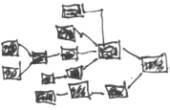
4) Algorithm spawns a copy of itself for each of the 3 additional pixels that have been detected up to this point per the illustration. The algorithm then generates a data structure, in nodal tree form, representing algorithmic replication and progression. Initial instance of Obj. recog. Algorithm now terminates. Each node represents an “on” pixel, as well as the termination of the associated algorithm instance. Each branching on the tree represents an instance replicating itself upon pixel detection and before instance termination. See below:

5) Analysis of nodal tree yields metadata on currently-examined pixel agglomeration. This analysis is recursive, with each traversal of a given tree branch triggering a more detailed analysis of current branch hierarchy level. Each node contains data relating to its nodal relationship to it’s parent and child

node(s), as well as it’s position on the pixel grid. See figure below:

6) Each tree branch will eventually come to an end. At branch termination, a tree “pruning” subroutine is launched. It iterates through the branch from end to beginning, cutting out redundant nodes and branchings. See below figures.

7) After all nodal tree branches have terminated, second level analysis of visual input is triggered, using the pixel grid of next-highest grayscale depth. All nodal points (“on” pixels) of first level output (the finished nodal tree) are correlated with their corresponding pixel on the higher depth pixel grid. If higher resolution grid has a depth of 64 gray shades, 1 being lightest, nodal points will correspond with pixels that posess a gray value >= 32. Nodes w/ values nearest to 32 are analysed for neighboring pixels of similarly low value; this is done in order to tentatively separate the 1^st level tree into multiple 2^nd level trees, each of which represents an significant, contiguous area of the visual input. See figures below.

7a) 2^nd level trees are statistically analysed w/ respect to various quantifiable patterns and features. An example of such might be analyzing the object’s perimeter’s fractal dimension. The results of said statistical analysis are compared to archived nodal tree patterns, in the first step towards tentative identification of analyzed object. See below.